Learning Objectives

Following this assignment students should be able to:

• Download global climatic data
• Download geographic occurrence data for a particular species
• Manipulate rasters
• Create spatial point dataframes
• Plot rasters and occurrences

---

Exercises

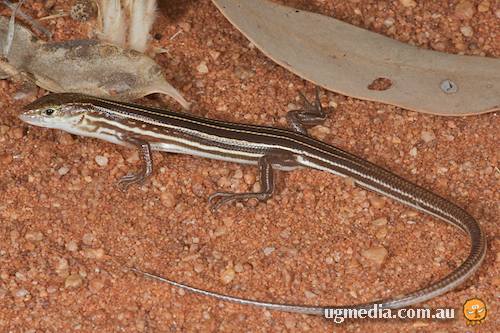
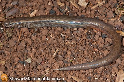
In this assignment, we are going to compare the climatic conditions of the habitats of two species of lizards in Australia, Ctenotus piankai and Calyptotis scutirostrum.

Before you start the assignment, accept the assignment repository here and clone it to your local machine. Make sure to commit and push any significant change.

Using the Intro to Spatial Analysis tutorial as reference,

1. Download the global climatic data from the Worldclim database using a resolution of 10m.
2. Download the geographic occurrence data from the two species of lizards from GBIF.
3. Using the mean annual temperature (bio1) and mean annual precipitation (bio12) rasters, calculate the Global Net Primary Production (NPP) using the Miami model
4. Extract the mean annual temperature, precipitation and net primary productivity values for each occurrence location in each lizard species. Before extracting the values, make sure to filter any NAs, zeros and duplicates from your lat and lon coordinates.
5. Plot a map of NPP in Australia displaying the occurrences of both lizards species in different colours (hint! use the argument add=TRUE to add a new layer to your plot).
   • You can use the function drawExtent() to extract the extent of Australia. However, you will need to write the values in a separate object, and then comment the line once you used the function. Using only the drawExtent() will affect the reproducibility of your code
6. Plot the distribution of the temperature and precipitation for each of the species of lizards.
7. Compare the distribution of NPP values for both lizard species using only one plot (check here for some examples)

Want a challenge?

• Instead of using histograms to compare the distribution of NPP, precipitation and temperature for both lizard species, use violin plots